West Antarctic Ice Sheet (WAIS)

This is our first real world example. We produce a map of approximate ice velocity in West Antarctica. This example demonstrates:

the capability of WAVI.jl in real world examples
how to specify the solution mask h_mask, which defines which grid points are part of the ice domain.
how to specify a spatially variable initial ice viscosity

NB the files included here are intended as a full demonstration of WAVI.jl capability, but should not be interpreted as "ready to go" for scientific inquiry; please get in touch if you would like to use these files for science!

Install dependencies

First let's make sure we have all required packages installed. We're also going to use the Downloads package to pull some data from a Github repository.

using Pkg
Pkg.add("https://github.com/RJArthern/WAVI.jl")
Pkg.add(Plots)
Pkg.add("Downloads")
using WAVI, Plots, Downloads

Reading in data

First, let's define our grid sizes and origin. We have a grid with 164 cells in the x direction and 192 in the y direction, with 5km resolution. We're going to use 12 levels in the vertical: even though WAVI.jl is designed for the solution of depth integrated equations, it retains some information about the vertical direction e.g. in the calculation of the ice viscosity; the keyword argument nσ, which is passed to a Grid object, specifies the number of levels in the vertical. We refer to the extension of the 2D (horizontal) grid to n$\sigma$ levels in the vertical as the 3D grid, which has size nx $\times$ ny $\times$ n$\sigma$.

nx = 164        #number of x grid points
ny = 192        #number of y grid pointd
nσ = 12         #number of sigma grid points
x0 = -1802500.0 #origin of the grid in x
y0 = -847500.0  #origin of the grid in y
dx = 5000.0     #grid resolution in x
dy = 5000.0     #grid resolution in y

We're going to download and read in the following data files:

h_mask : array of zeros and ones defining the ice domain (zero corresponds to out of domain, one to in domain).
u_iszero : location of grid points with zero velocity in x, effectively a boundary condition
v_iszero : location of grid points with zero velocity in y, effectively a boundary condition
bed : the bed elevation, which is a processed form of data from Bedmachine V3.
h : ice thickness , defined on the 2D grid
viscosity : the initial ice viscosity, defined on the 3D grid

We'll download them from GitHub, where they're stored in an external repo

We need the first three of these before we can build a grid:

h_mask=Array{Float64}(undef,nx,ny); #initialize mask array
read!(Downloads.download("https://github.com/alextbradley/WAVI_example_data/raw/main/WAIS/Inverse_5km_h_mask_clip_BedmachineV3.bin"),h_mask); #download the file and populate the h_mask array (can ignore the filename)
hm = ntoh.(h_mask); #set to big endian
hm = map.(Bool, round.(Int, hm)); #map everything to a boolean

u_iszero=Array{Float64}(undef,nx+1,ny);
read!(Downloads.download("https://github.com/alextbradley/WAVI_example_data/raw/main/WAIS/Inverse_5km_uiszero_clip_BedmachineV3.bin"),u_iszero);
u_iszero.=ntoh.(u_iszero);
u_iszero = map.(Bool, round.(Int, u_iszero));

v_iszero=Array{Float64}(undef,nx,ny+1);
read!(Downloads.download("https://github.com/alextbradley/WAVI_example_data/raw/main/WAIS/Inverse_5km_viszero_clip_BedmachineV3.bin"),v_iszero);
v_iszero.=ntoh.(v_iszero);
v_iszero = map.(Bool, round.(Int, v_iszero));

Now that we have these, we can build a grid:

grid = Grid(nx = nx, ny = ny, nσ = nσ, x0 = x0, y0 = y0, dx = dx, dy = dy, h_mask = hm, u_iszero = u_iszero, v_iszero = v_iszero)

Before moving on, let's have a look at the h_mask (i.e. which grid points are in the domain) using the spy function, which indicates which entries of a matrix are non-zero:

Plots.spy(hm)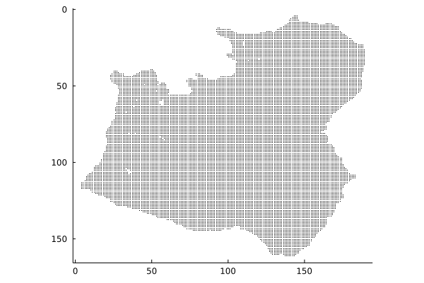

Those familiar with it will recognise the ice fronts of Pine Island, Thwaites and Smith ice shelves and the drainage basins of their glacies. For those not familiar, trust me: this is a rough outline of the Amundsen sea sector of West Antarctica!

Next up: the bed, which will be passed to a model via the bed_elevation keyword article:

bed=Array{Float64}(undef,nx,ny);
read!(Downloads.download("https://github.com/alextbradley/WAVI_example_data/raw/main/WAIS/Inverse_5km_bed_clip_noNan_BedmachineV3.bin"),bed);
bed.=ntoh.(bed)

Let's take a look at the bed

plt = Plots.heatmap(grid.xxh[:,1]/1e3, grid.yyh[1,:]/1e3, bed', 
                    xlabel = "x (km)", 
                    ylabel = "y (km)",
                    colorbar_title = "bed elevation (m)",
                    title = "West Antarctica bed elevation",
                    framestyle = "box")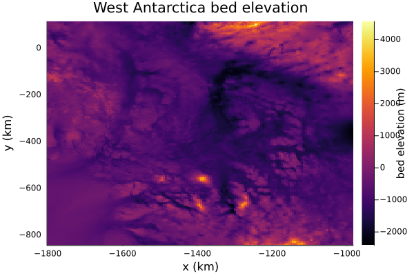

It's a little hard to see here, but the bed gets deeper towards the right of the plot, which is the direction of retreat of Thwaites and Pine Island Glaciers. This might lead to feedbacks which promote their retreat (the so-called 'marine ice sheet instability')

Initial temperature, damage, viscosity, and thickness will be passed to a model via initial conditions (these quantities are time dependent and would evolve with the simulation)

temp=Array{Float64}(undef,nx,ny,nσ);
read!(Downloads.download("https://github.com/alextbradley/WAVI_example_data/raw/main/WAIS/Inverse_5km_3Dtemp_clip_noNan_BedmachineV3.bin"),temp)
temp.=ntoh.(temp)

damage=Array{Float64}(undef,nx,ny,nσ);
read!(Downloads.download("https://github.com/alextbradley/WAVI_example_data/raw/main/WAIS/Inverse_5km_damage3D_clip_noNan_BedmachineV3.bin"),damage)
damage.=ntoh.(damage)

h=Array{Float64}(undef,nx,ny);
read!(Downloads.download("https://github.com/alextbradley/WAVI_example_data/raw/main/WAIS/Inverse_5km_thickness_clip_noNan_BedmachineV3.bin"),h);
h.=ntoh.(h)

viscosity=Array{Float64}(undef,nx,ny,nσ);
read!(Downloads.download("https://github.com/alextbradley/WAVI_example_data/raw/main/WAIS/Inverse_5km_viscosity3D_clip_noNan_BedmachineV3.bin"),viscosity)
viscosity.=ntoh.(viscosity);

initial_conditions = InitialConditions(initial_thickness = h,initial_viscosity = viscosity,initial_temperature = temp,initial_damage = damage)

Ice Velocity

#Now we're ready to make our model, which we can then use to determine the ice velocity. We'll let all physical and solver parameters take their default values by not passing a Params or SolverParams object to the model.

model = Model(grid = grid, bed_elevation = bed,initial_conditions= initial_conditions)

We use the update_state! method to bring fields (including velocity) in line with the ice thickness (note, this may take a few mins!)

update_state!(model)

Now we can visualize the ice velocity, which is stored in the model fields via model.fields.gh.av_speed:

plt = Plots.heatmap(grid.xxh[:,1]/1e3, grid.yyh[1,:]/1e3, model.fields.gh.av_speed', 
                    xlabel = "x (km)", 
                    ylabel = "y (km)",
                    colorbar_title = "ice speed (m/yr)",
                    title = "West Antarctica ice speed",
                    framestyle = "box",
                    clim=(0,4000))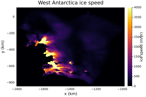

Ice velocities on ice shelves can be above 5km/yr! Inland, they're smaller.

If you wanted, you could evolve the ice thickness by setting up a Simulation object. You can find details on how to set up timestepping in other examples.