Planar One-Dimensional Flow
This a WAVI.jl's simplest example: flow down a flat plane in one horizontal dimension. This example demonstrates how to:
- load
WAVI.jl - instantiate an
WAVI.jlmodel - update ice velocities
- output solutions
- time-step a model forward
- look at results
Install dependencies
First let's make sure we have all required packages installed.
using Pkg
Pkg.add(PackageSpec(url="https://github.com/RJArthern/WAVI.jl.git", rev = "main"))
Pkg.add("Plots")
using WAVI, Plots
Instantiating and configuring a model
We first build a WAVI model, by passing it a grid containing information about the problem we would like to solve.
Below, we build a grid with 300 grid points in the x direction. We use 2 grid points in the y direction which is equivalent to being one-dimensional. This grid has a resolution of 12km.
grid = Grid(nx = 300, ny = 2, dx = 12000.0, dy = 12000.0)Next, we write a function which defines the bed (note that WAVI.jl accepts both functions and arrays of the same size as the grid as bed inputs, but here we'll use a function for simplicity). You can read more about functions in julia here
function bed_elevation(x,y)
    B = 720 - 778.5 * x ./ (750e3)
return B
end
This bed drops a height of 778.5m in every 750km, where the latter is a typical length scale for the Antarctic ice sheet.
Next we specify physical parameters via a Params object. In this case, we set the accumulation rate (the net snowfall) and leave all other parameters at their default values.
params = Params(accumulation_rate = 0.3);Let's also set the initial thickness (i.e. at the start of the simulation) of the ice to be 300m everywhere. Initial conditions in WAVI are set via InitialConditions objects:
initial_conditions = InitialConditions(initial_thickness = 300. .* ones(grid.nx, grid.ny));Now we are ready to build a Model by assembling these pieces:
model = Model(grid = grid, bed_elevation = bed_elevation, params = params,initial_conditions=initial_conditions);Updating the model state
Having built the model, we can solve for the ice velocities associated with the geometry we set via the initial conditions. To do so, we use the update_state! function, which takes a model and updates the velocities to be in line with the geometry.
update_state!(model)Visualizing the solutions
Now let's plot the ice profile and ice velocity, starting with the bed. We'll use julia's Plots.jl package to plot. Note that we make plot objects sequentially, and then use the display command to show them.
ice_plot = plot(model.grid.xxh[:,1]/1e3, model.fields.gh.b[:,1],
                linewidth = 2,
                linecolor = :brown,
                label = "bed",
                xlabel = "x (km)",
                ylabel = "z (m)");
Then we add the ice surface...
plot!(ice_plot, model.grid.xxh[:,1]/1e3, model.fields.gh.s[:,1],
                linewidth = 2,
                linecolor = :blue,
                label = "ice surface");
...and finally the ice base
plot!(ice_plot, model.grid.xxh[:,1]/1e3, model.fields.gh.s[:,1] .- model.fields.gh.h[:,1],
                linewidth = 2,
                linecolor = :red,
                label = "ice base");

display(ice_plot)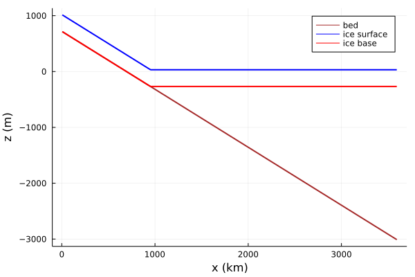
We see that the ice shelf goes afloat when the ice base is approximately 270m below sea level, which fits which Archimedean floatation principles: 270m is the product of the ratio of the densities of ice (about 900 km/m^3) and ocean (about 1000 kg/m^3) with the ice thickness (300m).
Now lets have a look at the velocity in the ice. We'll make a new plot for this:
vel_plot = plot(model.grid.xxh[:,1]/1e3, model.fields.gh.u[:,1],
                linewidth = 2,
                label = "ice velocity",
                xlabel = "x (km)",
                ylabel = "ice velocity (m/yr)");
display(vel_plot)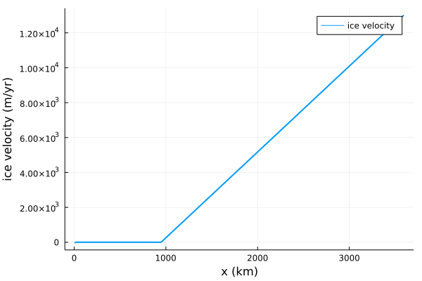
We see that ice velocities are very small (but non-zero, although not obvious from the plot) in the grounded ice, where friction between the ice and the bed restrains the flow. In the shelf, where there is no basal friction, velocities increase linearly to a maximum of 12km/yr (very fast!) at the downstream end of the shelf.
Advancing in time: running a simulation
Now, let's think about advancing time. To do so, we set up a simulation via a Simulation object, which can be time-stepped to advance the simulation and also manages output.
First we define a TimesteppingParams object, which holds parameters related to timestepping. Let's set the model to run for 10 years with a timestep of 0.5 years:
timestepping_params = TimesteppingParams(dt = 0.5, end_time = 100.);(Note that the end time end_time and timestep dt must be floating point numbers – we're working on fixing this!). Now we can build the Simulation object...
simulation = Simulation(model = model, timestepping_params = timestepping_params);...and run it, which will timestep the solution for 100 years
run_simulation!(simulation);Our simulation ran! The object simulation holds all the information about the state at time 10 years. Note that the current model state can be accessed via simulation.model, so we could use the above plotting commands to look at the geometry and velocity, if we wanted.
Outputting the solution
#Our simulation ran successfully, but we don't have any information about what happened. We get around this by outputting the solution regularly. To do so, we first make a clean folder where solution files will go:
folder = joinpath(@__DIR__, "planar_one_dimensional_flow"); #specify the location of the directory, @__DIR__ is the directory holding this script
isdir(folder) && rm(folder, force = true, recursive = true); #delete this folder (probably not good practice)
mkdir(folder) #make the folder
What to output and when to output it is specified by an instance of an OutputParams objects. Let's set one up so that the ice thickness, (unchanging) bed, ice surface and ice velocity is output every year, including at the first timestep:
output_params = OutputParams(outputs = (h = model.fields.gh.h,u = model.fields.gh.u, b = model.fields.gh.b,s = model.fields.gh.s), #which fields to output
                            output_freq = 10.,    #how frequently to output
                            output_path = folder, #where to store the results
                            output_start = true); #flag to output the state before the first timestep
Note that the outputs keyword argument takes a named tuple, which points to the locations of fields that are to be outputted. As in the timestepping_params, the output frequency must be a floating point number.
Let's build a new simulation, which knows about the outputting via the OutputParams object
simulation = Simulation(model = model, timestepping_params = timestepping_params, output_params = output_params)...and run it (nb this might take a few mins, depending on the spec of your pc!)
run_simulation!(simulation)The simulation will run and output the results as it goes.
Visualizing the results
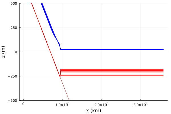
Let's look at how the shape of the ice sheet changes during the simulation. We'll plot the surface elevation for each of the output files (i.e. every 10 years). To do so, we first have to fetch the results: we'll loop over the output files and put the thickness and surface info a matrix
files = [joinpath(folder, file) for file in readdir(folder) if endswith( joinpath(folder, file), ".jld2") ] ;
nout = length(files);
h_out = zeros(simulation.model.grid.nx, nout);
surface_out = zeros(simulation.model.grid.nx, nout);
base_out = zeros(simulation.model.grid.nx, nout);
t_out = zeros(1,nout);

for i = 1:nout
    d = load(files[i]);
    h_out[:,i] = d["h"][:,1];
    base_out[:,i] = d["s"][:,1] .- d["h"][:,1];
    surface_out[:,i] = d["s"][:,1];
    t_out[i] = d["t"];
end
Now lets make the plot.
pl = Plots.plot(simulation.model.grid.xxh[:,1], simulation.model.fields.gh.b[:,1],
                    linecolor = :brown,
                    xlabel = "x (km)",
                    ylabel = "z (m)",
                    legend = :none,
                    ylim=(-500,500))
Plots.plot!(pl,simulation.model.grid.xxh[:,1], surface_out, legend = :none, linecolor = :blue)
Plots.plot!(pl,simulation.model.grid.xxh[:,1], base_out, legend = :none, linecolor = :red)
As time proceeds, the ice sheet accelerates, causing thinning.
Finally, we clear up the files we just outputted
rm(folder, force = true, recursive = true);