Numerical Implementation

Numerical Grid

WAVI.jl solves the governing equations on a rectangular grid, with $n_x$ grid cells in the $x$ direction and $n_y$ grid cells in the $y$ direction. Ice thickness values $h$ are defined at the cell centers (see figure) of grid cells, while velocity components $\bar{u}$ and $\bar{v}$ are defined along grid cell edges, and shear strain rates $c = (\partial u /\partial y + \partial v / \partial x)/2$ are stored at grid corners.

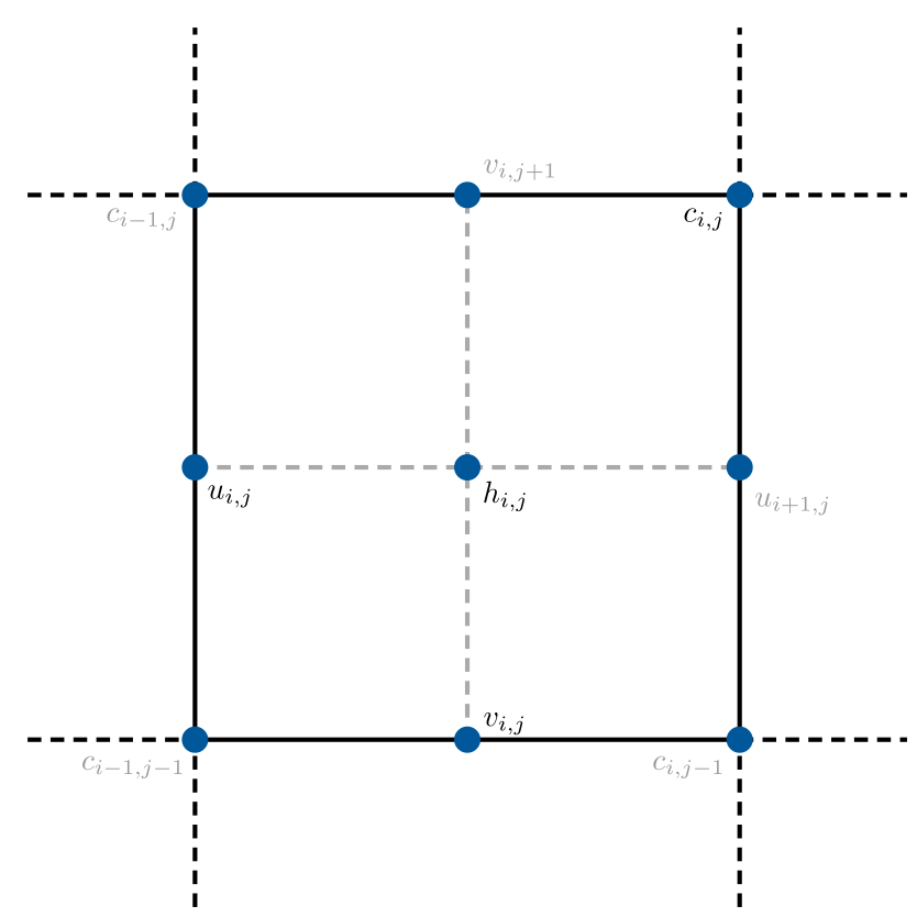
The set of all such points at which the ice thickness is stored defines the $h$-grid. The $u$-grid, $v$-grid, and $c$-grid are defined analagously. Various different quantities are also stored on each of these grids, and used as part of the solution (see Fields for more information).

Three dimensional fields used in the governing equations (e.g. viscosity) are stored $h$-grid points, extrapolated into the $z$ direction. This grid is referred to as the $\sigma$-grid.

Problem Reduction

This section contains brief details of the procedure by which the momentum balance equations governing equations(2)–(4) are reduced to a non-linear equation for the depth average velocity $\bar{\mathbf{u}}$. For full details, refer to [7].

To make progress in solving the governing equations, horizontal gradients in vertical velocity are neglected and vertical shear stresses are assumed to vary linearly with depth. Then, if the ice thickness $h$, surface elevation $h$, ice stiffness, basal stresses and horizontal stress components are known, the depth integrated viscosity

\[\begin{equation} \bar{\eta} = \frac{1}{h}\int_{s - h}^{h} \eta~\mathrm{d}z \end{equation}\]

can be computed numerically. Here $\eta$ is the ice viscosity (equation (4) in thegoverning equations).

After depth integrating the approximation to the horizonal stress components, and using the Robin boundary condition (equation (7)), the basal velocity components – and thus basal stress terms – can be expressed in terms of the depth averaged velocity components. The basal stress components can then be eliminated from governing equations(2)–(3), which can therefore be expressed as a non-linear problem for $\bar{\mathbf{u}}$, the depth averaged velocity:

\[\begin{equation} \mathcal{L}(\bar{\mathbf{u}}) \bar{\mathbf{u}} = \mathbf{f} \end{equation}\]

where

\[\begin{equation}\label{E:operator_problem} \mathcal{L} = \begin{pmatrix} \partial_{x} 4 \bar{\eta} h \partial_{x} + \partial_{y} \bar{\eta} h \partial_{y} - \beta_{\text{eff}} & \partial_{x} 2 \bar{\eta} h \partial_{y} + \partial_{y} \bar{\eta} h \partial_{x} \\ \partial_{x} \bar{\eta} h \partial_{y} + \partial_{y} 2 \bar{\eta} h \partial_{x} & \partial_x \bar{\eta} h \partial_x + \partial_y 4 \bar{\eta} h \partial_y - \beta_{\text{eff}} \end{pmatrix} \end{equation}\]

with $\beta_{\text{eff}}$ an effective drag coefficient (see equation (12) in [7]).

Velocity Solve

This section described very briefly the steps involved in the procedure by which the non-linear elliptic problem for the velocity (equation \eqref{E:operator_problem}) is solved in WAVI.jl. Again, for full details, refer to [7].

• The problem \eqref{E:operator_problem} is discretized with a finite difference approximation. Details of the discretization are included in the appendix of [7].
• The resulting problem is expressed as a symmetric saddle point problem.
• The saddle point problem is expressed as two distinct problems. The first is solver iteratively using a BiCGSTAB method
• The second problem is solved using an iterative method, leveraging an [LU-factorization] of the mass matrix in the problem.

Timestepping

If the system is to be solved forwards in time, the velocity must be solved simultanously with the surface elevation (i.e. equations (2)–(4) and (8)) must be solved simultanously. The procedure is largely as described above for the velocity components, but the problem is preconditioned using an iterative approach inspired by [8] to improve computational speed. Once the velocities have been solved for, the surface elecation is updated using a simple Euler scheme.