MISMIP+ example (part 2)
In this example, we demonstrate the retreat experiments performed in the Marine Ice Sheet Model Intercomparison (MISMIP) (doi: 10.5194/tc-14-2283-2020). There experiments are as follows: starting from a steady state determined in MISMIP+ part 1, we enforce melt induced for 100 years (this is called the ice1r experiment in MISMIP+) followed by no melting for 100 years.
This example demonstrates how to: * apply simple parametrizations of ice shelf basal melting * chain simulations via ice thickness
Install dependencies
First let's make sure we have all required packages installed. As well as WAVI and Plots for plotting, we're going to use the Downloads package to pull some data from a Github repository.
using Pkg
Pkg.add(PackageSpec(url="https://github.com/RJArthern/WAVI.jl.git", rev = "main"))
Pkg.add("Plots"), Pkg.add("Downloads")
using WAVI, Plots, Downloads
Setting up the model
Much of the model setup is as in the MISMIP+ example; this is contained in the code below (see the MISMIP+ part one for details):
dx = 8.e3;
dy = 8.e3;
nx = round(Int, 640*1e3/dx);
ny = round(Int, 80*1e3/dx); #fix the number of grid-cells in the x and y directions to match set extents
u_iszero = falses(nx+1,ny); #build x-direction velocity boundary condition matrix with no zero boundary conditions anywhere
u_iszero[1,:].=true;        #set the x-direction velocity to zero at x = 0.
v_iszero=falses(nx,ny+1);   #build x-direction velocity boundary condition matrix with no zero boundary conditions anywhere
v_iszero[:,1].=true;        #set the y-direction velocity to zero at y = 0 (free slip)
v_iszero[:,end].=true;       #set the y-direction velocity to zero at y = 84km (free slip)
v_iszero[1,:].=true;         #set the y-direction velocity to zero at x = 0km (no slip in combination with u_iszero)
grid = Grid(nx = nx,
            ny = ny,
            dx = dx,
            dy = dy,
            u_iszero = u_iszero,
            v_iszero = v_iszero)
params = Params( accumulation_rate = 0.3);
However, here we use a different initial condition (namely, the ice thickness at the end of the MISMIP ice0 experiment) and apply melting. We also don't reduce the number of iterations in the velocity solve (see MISMIP+ part one), because we want the velocity to converge at each timestep.
To save time, we'll pull the initial condition from GitHub ( where it has been saved), rather than running the first experiment again.
h_init=Array{Float64}(undef,nx,ny);
read!(Downloads.download("https://github.com/alextbradley/WAVI_example_data/raw/main/MISMIP_PLUS/MISMIP_ice0_steadythickness_8km.bin"),h_init)

initial_conditions = InitialConditions(initial_thickness = h_init)
Next we apply the parametrization of melting. In the MISMIP+ experiment, the melt rate on floating cells is $0.2 \tanh((z_d - z_b)/75) \max(-100 - z_d,0)$. We have hard-coded this melt rate into WAVI (you can find out more about how it is constructed in the melt parametrizations example); here, we just want to show how melt rate models are coupled to WAVI models.
First, we make the melt model...
melt_rate = MISMIPMeltRateOne()...and then pass it to the simulation by coupling it in the construction of the model
model = Model(grid = grid,
            bed_elevation = WAVI.mismip_plus_bed,
            initial_conditions = initial_conditions,
            melt_rate = melt_rate);
Retreat phase
In the ice 1r experiment, we run for 100 years with the melting applied. We need to define TimesteppingParams and OutputParams` objects to control timestepping and outputs respectively.
timestepping_params = TimesteppingParams(dt = 0.5,
                                        end_time = 100.,)

#make a folder for outputs
folder = joinpath(@__DIR__, "mismip");
isdir(folder) && rm(folder, force = true, recursive = true);
mkdir(folder) ;

#specify output parameters
output_params = OutputParams(outputs = (h = model.fields.gh.h,grfrac = model.fields.gh.grounded_fraction), #output the thickness and grounded fraction, so we can compute the volume about floatation
                            output_freq = 1., #output every year
                            output_path = folder,
                            zip_format = "nc");
Now we can make the simulation and run it
simulation = Simulation(model = model, timestepping_params = timestepping_params, output_params = output_params)
run_simulation!(simulation)
Let's plot the volume above floatation through time (volume above floatation is the volume of ice above the thickness set the Archimedean floatation condition).
filename = joinpath(folder, "outfile.nc");
h = ncread(filename, "h");
grfrac = ncread(filename, "grfrac");
time = ncread(filename, "TIME");
#compute the volume above floatation
vaf = zeros(1,length(time))
for i = 1:length(time)
    vaf[i] = volume_above_floatation(h[:,:,i], simulation.model.fields.gh.b, Ref(simulation.model.params), simulation.model.grid )
end
Plots.plot(time, vaf[:]/1e9,
             marker = true,
             label = :none,
             xlabel = "time (years)",
             ylabel = "volume above floatation (km^3)",
             framestyle = :box)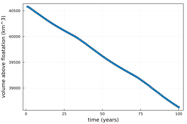
The volume above floatation decreases, indicating that the ice sheet is retreating. That's to be expected: the initial condition is in steady state with no melting, and the melting in this experiemnt is quite aggressive.
Advance phase
In the advance phase, we turn melting off. To chain this to the previous simulation, we use the thickness from the previous section as an initial condition.
initial_conditions_advance = InitialConditions(initial_thickness = simulation.model.fields.gh.h) #simulation.model.fields.gh.h is the current (i.e. after 100 years of simulation time) thickness of the retreat phase
model_advance = Model(grid = grid,
            bed_elevation = WAVI.mismip_plus_bed,
            initial_conditions = initial_conditions_advance) #note: no melt rate this time
We can use the same timestepping parameters. We'll make a new output parameters object so we can output in a different place
#make a folder for outputs
folder_advance = joinpath(@__DIR__, "mismip_advance");
isdir(folder_advance) && rm(folder_advance, force = true, recursive = true);
mkdir(folder_advance) ;

#specify output parameters
output_params_advance = OutputParams(outputs = (h = model_advance.fields.gh.h,grfrac = model_advance.fields.gh.grounded_fraction), #output the thickness and grounded fraction, so we can compute the volume about floatation
                            output_freq = 1., #output every year
                            output_path = folder_advance,
                            zip_format = "nc");
Now we can make the simulation and run it
simulation_advance = Simulation(model = model_advance, timestepping_params = timestepping_params, output_params = output_params_advance)
run_simulation!(simulation_advance)
Let's work out the volume above floatation evolution for this phase and add it to the earlier plot.
filename = joinpath(folder_advance, "outfile.nc");
h_adv = ncread(filename, "h");
grfrac_adv = ncread(filename, "grfrac");
time_adv = ncread(filename, "TIME");
time_adv = time_adv .+ time[end] #shift the time by the final entry of the retreat phase

#compute the volume above floatation
vaf_adv = zeros(1,length(time_adv))
for i = 1:length(time_adv)
    vaf_adv[i] = volume_above_floatation(h_adv[:,:,i], simulation_advance.model.fields.gh.b, Ref(simulation_advance.model.params), simulation_advance.model.grid )
end
Plots.plot(time, vaf[:]/1e9,
             marker = true,
             label = "advance",
             xlabel = "time (years)",
             ylabel = "volume above floatation (km^3)",
             framestyle = :box)

Plots.plot!(time_adv, vaf_adv[:]/1e9,
             marker = true,
             label = "retreat")