MISMIP+ example (part 1)

This example shows how to recreate the Marine Ice Sheet Model Intercomparison (MISMIP) (doi: 10.5194/tc-14-2283-2020) experiments. In this intercomparison exercise, a two-dimensional ice sheet is considered, with a grounding line that can stabilize on a section of bed which has a locally positive slope in the flow direction (commonly called retrograde). This is interesting because grounding lines on retrograde bedslopes are theoretically unstable in one horizontal dimension (see doi: 10.1029/2006JF000664), demonstrating the importance of variations in the second dimension for buttressing ice sheets. Note that here we use a very coarse (8km) resolution for computational speed. In this example, we demonstrate the MISMIP+ ice0 experiment, where the simulation is run to steady state with no melting; the other MISMIP+ experiments are shown in other examples.

This example demonstrates how to

apply boundary conditions
control the number of iterations in the velocity solve
zip the output into nc file format

Install dependencies

First let's make sure we have all required packages installed.

using Pkg
Pkg.add(PackageSpec(url="https://github.com/RJArthern/WAVI.jl.git", rev = "main"))
Pkg.add("Plots")
Pkg.add("NetCDF")
using WAVI, Plots

Basal Topography

The MISMIP+ domain is 640km in the x-direction and 80km in the y-direction, centred around $y = 0$. The basal topography is given by $z_b = \max [B_x(x) + B_y(y), -720]$ where $B_x(x)$ is a sixth order, even polynomial and $B_y(y)$ introduces two bumps in the domain. We write this analytic bed expression as a function

function mismip_plus_bed(x,y)
    xbar = 300000.0
    b0 = -150.0; b2 = -728.8; b4 = 343.91; b6 = -50.75;
    wc = 24000.0; fc = 4000.0; dc = 500.0;
    bx(x)=b0+b2*(x/xbar)^2+b4*(x/xbar)^4+b6*(x/xbar)^6;
    by(y)= dc*( (1+exp(-2(y-wc)/fc))^(-1) + (1+exp(2(y+wc)/fc))^(-1) );
    b = max(bx(x) + by(y), -720.0);
    return b;
end

First, let's take a look at this bed. First we'll use a nice high resolution grid to get a nice plot, but when we run the simulation, we'll use a lower resolution for computational efficiency

dx = 1.e3;
dy = 1.e3;
nx = round(Int, 640*1e3/dx);
ny = round(Int, 80*1e3/dx);
xx=[i*dx for i=1:nx, j=1:ny];
yy=[j*dy for i=1:nx, j=1:ny] .- 42000;
x = xx[:,1];
y = yy[1,:];

# Now we can plot
plt =  Plots.heatmap(x/1e3, y/1e3, mismip_plus_bed.(xx,yy)', 
                    xlabel = "x (km)", 
                    ylabel = "y (km)",
                    colorbar_title = "bed depth (m)")
plot!(size = (800,400))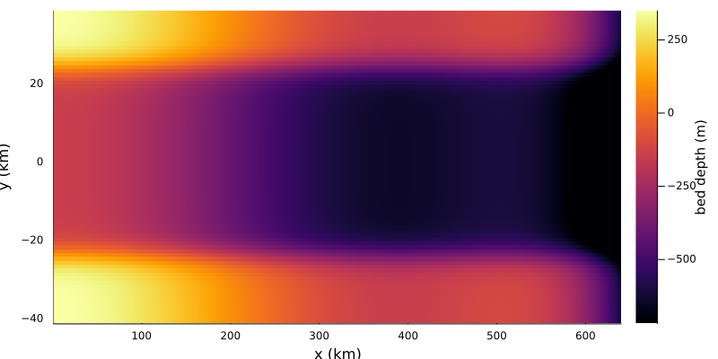

Boundary Conditions

In the MISMIP+ experiment, no slip (zero velocity in both directions) boundary conditions are applied at $x = 0$, and free-slip boundary conditions (zero velocity in the direction normal to the walls) are applied at the lateral boundaries at $y = 0$km and $y = 84$km. First, let's redefine the grid size to be lower resolution (to make the later simulations quicker)

dx = 8.e3;
dy = 8.e3;
nx = round(Int, 640*1e3/dx);
ny = round(Int, 80*1e3/dx); #fix the number of grid-cells in the x and y directions to match set extents

Velocity boundary conditions are controlled by specifying zeros in appropriate entries in arrays, which are then passed to the grid. We first build arrays, and then populate them with entries which enforce the boundary conditions:

u_iszero = falses(nx+1,ny); #build x-direction velocity boundary condition matrix with no zero boundary conditions anywhere 
u_iszero[1,:].=true;        #set the x-direction velocity to zero at x = 0.
v_iszero=falses(nx,ny+1);   #build x-direction velocity boundary condition matrix with no zero boundary conditions anywhere 
v_iszero[:,1].=true;        #set the y-direction velocity to zero at y = 0 (free slip)
v_iszero[:,end].=true;       #set the y-direction velocity to zero at y = 84km (free slip)
v_iszero[1,:].=true;         #set the y-direction velocity to zero at x = 0km (no slip in combination with u_iszero)

Now we build the grid as usual, passing the arrays we just constructed via optional arguments.

grid = Grid(nx = nx, 
            ny = ny,   
            dx = dx, 
            dy = dy,
            u_iszero = u_iszero, 
            v_iszero = v_iszero)

Solver Parameters

In the first MISMIP experiment, we're want to get to the final steady state, and don't really care about the solution state along the way. In particular, we don't need to get the velocity right along the way, we just want have it correct eventually. We therefore set the number of iterations in the velocity solve to be small: at each timestep, the solver just does a small number of iterations, and the velocity is only approximate. But, since we do a lot of iterations getting to steady state, the velocity gets to the right thing eventually. The number of iterations in the velocity solve and other parameters relating to how the equations are solved, are set via a SolverParams object:

solver_params = SolverParams(maxiter_picard = 1)

Explicitly, we set the number of iterations (formally, Picard iterations) to be as small as possible, i.e. one iteration.

Make the model

Now we have our grid, bed, and solver parameters, we just need to set the appropriate initial conditions and physical parameters for MISMIP+, and then we can build our model. In MISMIP+, the initial condition is 100m thick ice everywhere and the accumulation rate is 0.3m/a:

initial_conditions = InitialConditions(initial_thickness = 100 .* ones(nx,ny));
params = Params( accumulation_rate = 0.3);

Note that all other parameter values in WAVI have defaults set to the MISMIP+ values.

Now let's make our model! Note that we use the functional form of the bed:

model = Model(grid = grid,
            bed_elevation = mismip_plus_bed, 
            initial_conditions = initial_conditions,
            params = params, 
            solver_params = solver_params)

Assembling the Simulation

To get to steady state, we need to run our simulation for a good chunk of time, on the order of tens of 1000s of years. We'll run for 10000 years, with a timestep of half a year:

timestepping_params = TimesteppingParams(dt = 0.5, 
                                        end_time = 10000.,)

Note that as in other example, we have to specify the end time as 10000. (a float number) rather than 10000 (an integer) because WAVI.jl expects the same numeric type for the timestep dt and the end time end_time.

We'll output the solution along the way, and use this to convince ourselves later than we are in steady state. First let's make a directory to store the output

folder = joinpath(@__DIR__, "mismip");
isdir(folder) && rm(folder, force = true, recursive = true);
mkdir(folder) ;

Then we define our output parameters. We'll output the thickness and grounded fraction every 200 years, and set the zip_format keyword argument to zip the output files to an nc format when the simulation is finished.

output_params = OutputParams(outputs = (h = model.fields.gh.h,grfrac = model.fields.gh.grounded_fraction),
                            output_freq = 200.,
                            output_path = folder,
                            zip_format = "nc");

Now we assemble our simulation, taking in the model, output parameters and timestepping_params:

simulation = Simulation(model = model, timestepping_params = timestepping_params, output_params = output_params)

Timestepping

Now all that's left to do is run our simulation! This is a long simulation and might take a while (~10 mins on my laptop)

run_simulation!(simulation)

Visualization

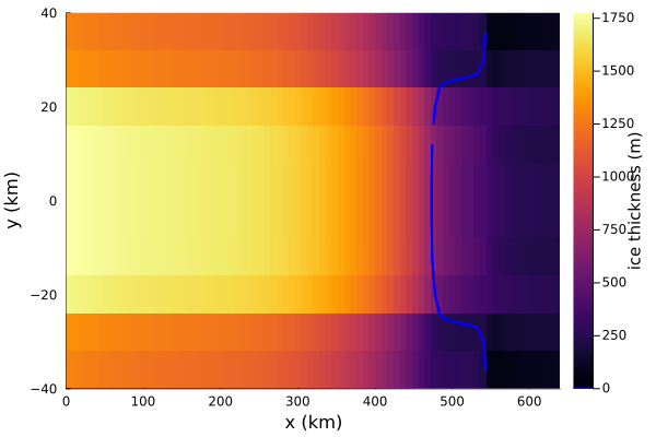
Let's have a look at the steady state thickness:

Plots.heatmap(simulation.model.grid.xxh[:,1]/1e3, simulation.model.grid.yyh[1,:]/1e3, simulation.model.fields.gh.h', 
                xlabel = "x (km)", 
                ylabel = "y (km)",
                colorbar_title = "ice thickness (m)")

And add the grounding line, which is where the grounded fraction transitions between 0 and 1 (grounded_fraction takes the value 1 at fully grounded grid points and 0 at fully floating grid points.) Our choice of 0.5 is somewhat arbitrary here – any value between 0 and 1 will do!

Plots.contour!(simulation.model.grid.xxh[:,1]/1e3, 
            simulation.model.grid.yyh[1,:]/1e3,
            simulation.model.fields.gh.grounded_fraction',
            fill = false,
            levels = [0.5,0.5],
            linecolor = :blue,
            linewidth = 2)
plot!(size = (1000,550))

You can see, by comparing with the plot of the bed earlier, that the grounding line sits on an overdeepened section of the bed! You can also compare it with the other MISMIP submissions (figure 3 in Cornford et al., 2020) and see that the grounding line position agrees pretty well with other models, despite being lower resolution.

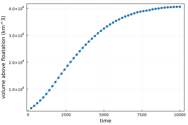
Finally, let's check that it's in steady state, by looking at the evolution of the volume above floatation:

filename = joinpath(folder, "outfile.nc");
h = ncread(filename, "h");
grfrac = ncread(filename, "grfrac");
time = ncread(filename, "TIME");
#compute the volume above floatation
vaf = zeros(1,length(time))
for i = 1:length(time)
    vaf[i] = volume_above_floatation(h[:,:,i], simulation.model.fields.gh.b, Ref(simulation.model.params), simulation.model.grid )
end
Plots.plot(time, vaf[:]/1e9,
             marker = true, 
             label = :none,
             xlabel = "time (years)",
             ylabel = "volume above floatation (km^3)",
             framestyle = :box)

The volume above floatation reaches a plateau, suggesting that we have indeed reached a steady state.

Finally, we clear up the files we just outputted

rm(folder, force = true, recursive = true)